Table of contents. 

1. Introduction. 

2. Paradigm: linear vs non-linear. 

3. Method for modeling the dynamics of value in the financial market. 

3.1. Foreword. 

3.2. The financial market is the NDASS. 

3.3. Cost is a function of time: P = N (T). 

3.4. Fractal and fractal structure. 

3.5. The order, views and types of fractals. 

3.6. Basic fractal. 

3.7. General view of the fractal structure. 

3.8. Basic fractal dynamics. 

3.9. Description of the fractal structure. 

3.10. Determination of order and chaos. 

3.11. The order of fractals. 

3.12. Numbering of fractals. 

3.13. Determination of extremum points. 

3.14. Views and types of fractals. 

3.15. 15 fractals: 

3.15.1. Fractals of the 1st view; 

3.15.2. Fractals of the 2nd view; 

3.15.3. Fractals of the 3rd view. 

3.16. Proportions between fractal segments. 

3.17. The Alphabet of Niro attractors. 

3.18. Bifurcation point and degrees of freedom. 

3.19. Cost and time intervals. 

3.20. The essence of the modeling method. 

4. Model of the future dynamics of the Dow Jones index values. 

5. Conclusion. 

This article describes a method for modeling the future dynamics of the value of financial assets. 

The method is based on chaos theory and fractal geometry. 

Apophenia is the ability to see structure, interconnection, regularity where they are not obvious or hidden. 

Everything is natural in the Universe. Regularity is present everywhere and in everything continuously. 

Regularity is always hidden, therefore the phrase "There is no regularity here!" says not about its absence, but about the fact that the pattern has not yet been discovered. The pattern is found only in the process of its search. 

The article describes the possibility of predicting the dynamics of the financial market and the method of modeling the dynamics of quotations of financial assets. 

The clairvoyance of the financial market is not about over-ability from the category of something over-natural. It is clear to see the future dynamics of quotations of currencies, stocks, bonds, futures and options for everyone. 

The task of modeling the dynamics of quotations is not more complicated than the task of solving a quadratic equation. The modeling method, like the method of finding the roots of a quadratic equation, presupposes the performance of an understandable algorithm of actions. 

A clear vision of the dynamics of the financial market follows from a clear vision in the chaotic fluctuations of the value of financial assets of the regular dynamics, structured in accordance with a certain order. 

1. Introduction.

The economic theory that developed in the last century, with the dominant linear paradigm, is unable to explain the processes occurring in the economy and does not allow predicting their future development, leaving unanswered the questions of the pricing mechanism in the capital markets.

The dynamics of value in the financial market, subject to sudden and sharp fluctuations, is not explained either by the efficient market hypothesis, or by any other hypotheses put forward by economists of the traditional classical school.

Studies of capital markets in the context of their functioning force us to look for new approaches to finding a pricing mechanism in which scientific knowledge will coincide with objective reality.

The need to introduce a new paradigm is becoming more and more obvious, in which the theory would explain the future dynamics of value in the financial market, and objective reality would confirm this. Just about such a theory describing the mechanism that brings the value in the financial market into dynamics will be discussed in this article.

Nonlinear dynamical systems, chaos theory, fractal geometry, synergetics - these are the directions of scientific thought that, in relation to the dynamics of value in the financial market, provide an explanation and understanding of what has happened, what is happening and what will happen with the dynamics of quotations of financial instruments.

The dynamics of the value of financial instruments, emerging in electronic trading and trading on stock exchanges, is not chaotic, because it is subject to a certain law that allows it to be predicted. Accordingly, the dynamics of the entire financial market is also predictable.

The forecasting method based on this law makes it possible to simulate the future dynamics of the value of financial assets and, on the basis of the compiled models, make effective investment decisions by actually managing market risk.

In a broader sense, it can be said that a forecasting method is a computational technology for modeling the behavior of nonlinear processes in social dynamic systems, which are financial markets as part of the economy.

Modeling the dynamics of the financial market assumes, based on the analysis of time series, to determine the models of the future dynamics of quotations of financial instruments (currencies, stocks, indices, derivatives, etc.), and then filter them in order to select the most probable development scenarios.

The model of the future dynamics of the value of a financial asset is a description of the most probable price movement trajectories on the chart, which are relevant at the time of compilation.

2. Paradigm: linear vs non-linear.

A paradigm is a speculative model that allows you to consider phenomena in a global aspect.

First, we will briefly consider the generally accepted theory of capital markets in a linear paradigm, indicating its advantages and disadvantages, and then we will outline the superiority of the nonlinear paradigm for describing the dynamics of the financial market.

The advantage of a linear model is its simplicity, so it is easier to work with linear models, turning a blind eye to the dangers of errors in calculations that lie in its limitations.

To make financial markets more understandable, economists have created explanatory models that do not fully reflect reality. With the help of a few simplifying assumptions about investor behavior, a general analytical model was created in a linear paradigm that does not work well, but explains some phenomena and processes in the economy, while leaving much unclear and inexplicable.

So, for example, it is found that economic forecasts have limited empirical validity, that is, the constructed economic models of the future reflect reality only in a short time interval, because a small change in only one variable has a huge impact on the future result.

Moreover, it is increasingly discovered that value in the financial market does not actually behave in the way required by the theory of random walks, which economists use in their calculations.

There are many more large price jumps in the markets to be explained by the exception to the rule in the form of noise effects.

At the stage of the emergence and development of econometrics as a science, the emergence of opportunities for accurate forecasting of the development of economic processes was assumed in order to prevent and avoid economic crises or their negative consequences.

Today, economic forecasts are often the object of mockery and ridicule, because there is no need to talk about any of their predictive effects.

Where do the errors come from, where do they lie, and why does modern economic theory not allow one to foresee crises in the economy in order to properly prepare for them? What are the problems?

First, one of the problems is the concept of equilibrium existing in economic theory. The econometric approach assumes that if there are no external influences, then the system is at rest, that is, in a state of equilibrium, in which everything balances each other. For example, supply equals demand.

The emerging exogenous factors, disturbing the system, throw it out of balance. The system reacts to the disturbance and returns to the equilibrium position linearly and immediately, because it always strives to be in equilibrium and does not accept imbalance. To maintain the concept of equilibrium, the concept of an efficient market was introduced, according to which all assets are valued fairly, i.e. using all the information that is available to all market participants without exception, who, moreover, are averse to risks in investment activities.

However, all these assumptions about equilibrium, about the general availability of information, about ignoring risks, to put it mildly, are far-fetched and do not correspond to the real state of affairs.

The market economy is an evolving system, attempts to control, manage and keep in balance are doomed to failure. With regular frequency, economic crises falling on us like snow on our heads are a good confirmation of this.

Secondly, time is an important problem for an econometric view of the world. Econometrics ignores time, i.e. economics and markets in this approach have no memory of the past or have a very limited memory. At its best, econometrics recognizes short memory. It is believed that memory effects dissipate rapidly.

The idea that one event can influence the future indefinitely is foreign to econometrics. The real state of affairs indicates the opposite. Absolutely all events that have ever happened in the past, regardless of the statute of limitations, have an impact on the development of the economy and the dynamics of the financial market in the present and the future - even a day ago, even a week ago, even a month ago, even years, decades and centuries ago.

Capital markets theory in a linear paradigm is based on the following concepts:

1. Rational investors.

Rational investors aim for an average return with a level of risk that is measured as a standard deviation. The preference is given to assets that give the highest expected return for a given level of risk. Investors are risk averse and avoid it in every possible way.

2. An efficient market.

An efficient market means that information is immediately reflected in prices, which are formed by all market participants who have equal access to it.

3. Random walks.

In accordance with the above two concepts, prices and, as a consequence of profit, follow a random walk, i.e. their probability distribution is normal, which means the possibility of applying the law of normal distribution of a random variable and calculating the mathematical expectation with variance.

The linear paradigm assumes that investors respond linearly to information, using it immediately after receiving it and not expecting it to accumulate in a series of subsequent events. The linear view follows the concept of the rational investor, which states that past information has already been discounted and reflected in prices. Thus, the linear paradigm implies that profits should be approximately normal and independent.

The non-linear paradigm considers all possible reactions of investors to information, both linear and non-linear, which increases the number of possible scenarios for the development of the situation.

The results of studies of time series of various financial assets show that prices do not follow a normal distribution, therefore, it is impossible to apply the theory of random walks to them and use the methods of statistical analysis in calculations.

Excessive value volatility in the markets challenges:

• the idea of rational investors;

• a concept stating that market efficiency can be achieved through a large number of market participants.

Random walk is necessary for applying statistical analysis to time series of price changes for portfolio theory to exist. Without a normal distribution in a linear paradigm, theoretical and empirical calculations are meaningless.

The efficient market theory is based on the postulate of rationality of investors. Rationality is determined by pricing based on all available information. Rationality also means that investors are risk averse. But are people rational in their totality as a whole, if we start from this definition of rationality? Of course not!

Consider how people react when faced with the choice of making a loss or a profit.

The generally accepted theory is that investors are risk averse. And if someone takes a big risk, then this risk must be compensated by the possibility of making a big profit.

Studies of all kinds show that when losses are acceptable, people take risks and become more like gamblers than rational investors.

Let's take an example to show the change in risk appetite.

Suppose an investor has a choice between:

1) Guaranteed earnings of $ 85'000 or

2) 85% opportunity to earn $ 100'000 and 15% opportunity to earn nothing.

Most investors would prefer a guaranteed return of $ 85,000, although the expected return is the same in both cases at $ 85,000. This choice confirms the risk aversion of investors.

If you offer to make a choice between:

1) Guaranteed loss of $ 85'000 or

2) 85% chances of losing $ 100'000 and 15% - not losing anything

then, despite the same expected loss in both cases, people will already take risks and the chance of avoiding losses will be preferable to the chance of incurring a guaranteed loss, even if the probability of this future loss is high. The wording has changed and now investors are looking to take risks.

Efficient market theory also assumes that all investors have the same investment horizon. This assumption is necessary in order for the expected returns to be comparable. But it is well known that in reality this is not the case.

When the opportunity to receive $ 10'000 now or $ 10'500 in a month is offered, most investors will prefer to receive $ 10'000 now. However, if investors are offered $ 10'000 in a year or $ 10'500 in 13 months, then most investors will choose a longer period of time to receive $ 10'500. Again, this does not fit the rational investor model.

Particular attention should be paid to how people behave in conditions of uncertainty. The rationality hypothesis of investors states that their subjective risk assessments are the same. However, the overwhelming majority of investors tend to be overconfident in their assessments and forecasts. The human brain is designed in such a way that it makes decisions with high certainty after receiving scanty information.

Confidence in decision making in the face of uncertainty is a standard situation for investors. However, overconfidence can lead to ignoring important information that could be used by others. Consequently, based on their subjective assessments, investors tend to assign greater likelihood to individual economic scenarios than is justified by real facts.

So, for example, if in some economic scenario 60% is assigned to growth, 30% to no growth, and 10% to recession, then in reality an investor who is confident in the growth scenario will prefer to increase this probability to 90%, and leave 10% for sluggish growth so as not to look too confident. As for the recession, it will be said that it is not possible at the moment.

Observations of investors show that they do not react and do not follow the trends that have begun in the markets until these trends are clearly manifested and established. Investors do not extrapolate the phenomena and events occurring in the markets for some time of their development, after which they make decisions that are conditioned by the accumulated information, ignored up to a certain point in time. This behavior of investors is fundamentally different from the intended actions of rational investors, who should immediately be guided by all new information.

Investors tend to be overconfident in their own predictions, so they ignore important information if it does not coincide with their opinion. Investors do not give up their forecasts until they receive enough information about a change in the situation.

If investors react in this way, then the market cannot be efficient because all information is not reflected in market prices. Much, in this case, remains unaccounted for in prices, and the reaction of investors to the events that have taken place comes later and there is no need to talk about any linearity.

When individual investors are not inclined to be so rational, then there is no reason to believe that this is not the case in the entire investing community.

If investors ignore information until trends are established, and then, taking into account all the accumulated information, use it in making decisions, this means that the reaction to information is non-linear. As soon as the amount of accumulated information exceeds a certain critical level, then all of its cumulative influence immediately begins to affect, which did not entail any consequences before. This speaks of the direct influence of the past on the present and, consequently, of the complete inconsistency of the efficient market theory, in which information and the response to it are in a rigid causal relationship, according to which the information received is immediately reflected in prices.

The rational investor concept and the efficient market hypothesis, based on the observation independence assumption and normal distribution, were created to apply probabilistic calculations in economic theory. The application of this concept in practice shows the fallacy of this simplifying assumption about a rational investor, because objective reality does not confirm the calculations and forecasts made.

In addition to the unrealistic nature of the rational investor, lack of public availability of information, and abnormal distribution, capital market theory with a linear paradigm ignores the assumption that different markets and different securities are related to each other.

Unlike linear systems, nonlinear dynamic systems are systems in the dynamics of which:

 there is a feedback, which means the dependence of what is happening in the present on what happened in the past;

 there are critical levels where there is more than one equilibrium position;

 dynamic fractals are formed;

 there is a sensitive dependence on the initial conditions.

All of the above indicates that financial markets are still nonlinear dynamic systems and then the following can be expected from them:

1. Long-term correlations and trends, i.e. feedback effects;

2. Variability with critical levels under certain conditions and at a certain time;

3. The presence of a fractal structure of time series;

4. Decrease in forecast reliability with increasing time intervals, i. E. manifestations of a sensitive dependence on the initial conditions.

The above is inherent in systems that are not equilibrium and typical for the markets that we know from experience and practice.

Efficient market theory in a linear paradigm is like cube-shaped clouds that can exist only in the heads of theorists who are out of touch with reality, whose economic forecasts will never be accurate because:

• Investors are not always risk averse. Very often, almost always, investors will be willing to take risks if they realize that without risk they are doomed to losses.

• Subjective assessments of investors are full of biases. They are much more confident in their own predictions than the available information warrants.

• Investors may not respond to information immediately upon receipt. Instead, they may respond to it some time later if it confirms a change in a recent trend, which suggests a non-linear response.

• There is no evidence and no evidence that investors are rational collectively than individually.

The dominance of the linear paradigm in relation to the financial market ceases, because the markets have clearly shown that they are rarely so ordered in our linear understanding of them, since very often, especially when the least expected, there is an exponential super-reaction to the impact, indicating nonlinearity of response than linearity.

Chaos theory and the sciences of nonlinear dynamical systems offer a different approach to describing what is happening in the financial market. To understand the past, be aware of the present and see the future in economics, it is necessary to change the linear paradigm to a nonlinear one. The old methods should be replaced by new ones that do not imply independence, rationality, random walks, and normal distributions.

Markets should be viewed as non-linear dynamic additive synergetic systems (NDASS), and the dynamics of value should be described by dynamic fractals. The non-linear paradigm must allow the concept of long-term memory into market theory, which postulates that events that have occurred can affect markets for an infinitely long time.

Changes in the quotes of financial instruments, if they do not fit into the economic theory with a linear paradigm, are usually explained by the selection of news that matches the logic, and if such news cannot be found, then everything remains without any explanation with the hope of future news that will fit into the logic of what happened.

Unlike the linear paradigm, the nonlinear paradigm always gives an answer to the question about the reasons for one or another price dynamics in the financial market, regardless of the financial instrument and the market on which it is traded.

It is time to end with the linear paradigm and move on to the rails of a non-linear paradigm, which offers the possibility of modeling the dynamics of value in the financial market.

3. Method for modeling the dynamics of value in the financial market.

3.1. Foreword.

Before proceeding directly to the consideration of the method of modeling the dynamics of value in the financial market, let us make a short introduction.

The theory of nonlinear dynamical systems was created to describe the motion of particle flows in physical media such as gas, liquid, plasma. When the magnitudes of external influences on the system, for example, temperature or pressure, change, the theory makes it possible to describe and simulate, in accordance with the parameters of external influences, the dynamics of flows passing in these media.

If the financial market has the properties of a nonlinear dynamic system, then a completely logical question arises - can the theory of nonlinear dynamic systems be applied to the description and modeling of the dynamics of the financial market? The answer is yes, you can!

Let's remember the definition of the concept "Finance".

Finance is a set of economic relations arising in the process of formation, distribution and use of centralized and decentralized funds of funds.

It follows from the definition that finances are cash flows, that is, finances are dynamics.

An economic system is analogous to a physical system, and there are particle flows here and there. In a physical system, such particles can be particles of gas, water, plasma, and in an economic system, such particles can be considered money in all their forms and manifestations.

An external influence on a physical system, for example, a change in such parameters as temperature, pressure, or both, leads to a change in the dynamics of flows in this system. Similarly, we can talk about an economic system, where under external influences, for example, such as a change in the interest rate, supply and demand, the rate of profit in some industry, etc., there is a change in the dynamics of cash flows, which change directions moving both inside both outside the local market and between various other markets - foreign exchange, stock, commodity, raw materials, that is, inside the all-embracing financial market.

Financial markets represent cash flows in the economy and these cash flows are not uniform, they can be characterized as turbulent and chaotic by analogy with the flows generated in various physical systems.

The generator of the simplest cash flow is a person as a subject of economic relations, who is influenced by his environment, including the information field.

Each person has a certain amount of money that came to him in the form of salaries, benefits, dividends, interest and other income from sources that cannot be listed. Spending his money, a person, without realizing it, generates certain cash flows. These cash flows of people individually are hardly noticeable and not perceptible, they are like drops of water, from which formed thin streams pour into streams, then with streams into rivers, from rivers to seas and further into oceans, followed by evaporation and transformations again into drops.

Cash flows generated by hundreds, thousands, millions of people are already becoming visible and tangible. For example, the demand for Apple's products has generated colossal cash flows that have managed to dramatically raise the company's market capitalization.

In general, the financial market is a nonlinear dynamic system with uneven cash flows, which means that to describe the dynamics of the financial market, you can use all the tools that are only applicable to nonlinear dynamic systems.

In physical systems, the number of external influences is a finite number. If we speak in the language of mathematics, then an external influence is understood as a certain variable. With a finite number of variables, it is possible to introduce the concept of a function that describes the dependence of the flow dynamics on changes in these variables, and the dependence itself can be expressed through an equation that has a finite number of solutions.

For example, the presence in a physical system of two external influences on it in the form of temperature and pressure makes it possible to represent the rate of flow change as a function of these two variables.

But an economic system is far from being a physical system in which you can experiment an infinite number of times, changing the parameters of external influences and finally bring this system back to its original state.

The financial market is a system that has no finite number of external influences. Everything from the discount rate to unverified rumors can be external influences.

We can say that the value in the financial market is a function of an infinite number of external influences, which are independent variables:

P = F(x1, x2, x3, …, xn)

where

P is the price of a financial asset;

Xn is external influence, n → ∞.

The solution to this equation, i.e. finding the value of the future value of a financial asset, in this formulation of the problem, is not possible.

A different approach is needed.

Recall that the solution to a quadratic equation can be found not only by formulas from the equation of a function, but also by the graph of this function.

The approach, in which the solution to an equation can be found graphically, is applicable to nonlinear dynamical systems.

For this, we will make several assumptions.

Cash flows are expressed in terms of value. So, the dynamics of cash flows between economic entities is reflected in the financial statements of these entities, but on a more global scale - in the trade balances of countries. The dynamics of cash flows in the financial market is reflected in the dynamics of the value of financial assets.

Organized markets (exchanges, electronic trading platforms), in conjunction with information technologies, give us a unique opportunity in real time to monitor the dynamics of cash flows in the foreign exchange, stock, commodity, raw materials markets, both in a particular region and in the global world.

Let's consider the mechanism of formation of prices of financial instruments in the organized market.

Investors wishing to buy or sell something place appropriate orders to buy or sell certain financial assets.

The volumes of orders put up for purchase at a specific price, exceeding the volumes of orders put up for sale at the same price, at a certain point in time move the price of this financial asset upwards. And vice versa, the volumes of orders put up for sale at a specific price, exceeding the volumes of orders put up for purchase at the same price, at a certain point in time move the price of the financial asset down.

Thus, we can say that only one single factor affects the price of a financial asset, namely, orders placed by investors in the order book. Only placed and executed orders move prices down or up.

In this case, all organized markets, which include all participants in the process - from regulators and organizers of trades to buyers and sellers on which financial instruments are traded, can be conventionally considered some kind of black boxes, at the exit from which, through a glass, as a kind of measuring device, readings of quotes are recorded at each specific moment in time. The readings from the order book plotted on the chart will describe the dynamics of cash flows.

Simplifying everything as much as possible, the graph of the change in cost over time can be represented as a graph of the function N, which is an operator that specifies the correspondence between the set of values of P and the set of values of T:

P = N (T)

where

P is the price of a financial asset;

T is time.

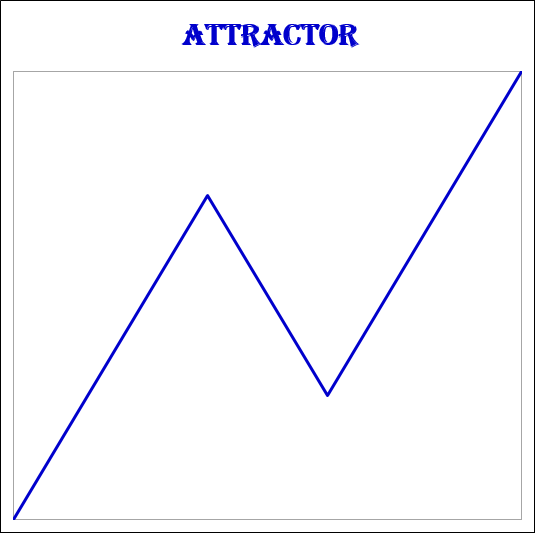
Taking into account that this is a graph of a nonlinear function describing the dynamics of a nonlinear dynamic system, we can say that the graph is an attractor, the structure of which is formed by dynamic fractals.

To move on, you need to brush up on some concepts and their definitions.

Dynamic system.

A dynamic system is understood as a process for which the concept of a state is uniquely defined as a set of values of some quantities at a given moment in time and an operator is given that determines the evolution of the initial state in time.

Attractor.

Attractor (English attract - to attract, to attract) is a compact subset of the phase space of a dynamical system, all trajectories from some neighborhood of which tend to it at time tending to infinity. An attractor can be a periodic trajectory or some bounded region with unstable trajectories inside in the case of a strange attractor.

A strange attractor.

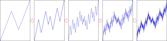
The peculiarity of a strange attractor lies in its scale invariance, which is expressed in the fact that when the scale of a certain subdomain of a strange attractor is increased or decreased, a geometric object is obtained, which is similar in structure to the whole attractor.

Phase space.

The phase space of a system is a collection of all admissible states of a dynamic system. Thus, a dynamic system is characterized by its initial state and the law according to which the system passes from one state to another.

Bifurcation point.

A bifurcation point is a critical state of a dynamical system, at which the system becomes unstable with respect to fluctuations occurring in it, and uncertainty arises: will the state of the system remain chaotic or it will move to a new, higher level of order.

Chaos.

Chaos is a non-repetitive, irregular, disorderly sequence of states of a dynamical system or the disorderly behavior of the attractors of this system.

Fractal.

A fractal is a structure consisting of parts that are similar to a whole. It can also be said that a fractal is an attractor of a nonlinear dynamical system.

Dynamic fractal.

Dynamic fractals describe the dynamics of processes occurring in time in nonlinear dynamic systems. In its development, a nonlinear dynamic system passes through alternating stages of a stable and chaotic state, as a result of which ordered states arise from chaos, which bring the system back to a chaotic state.

Synergetics.

Synergetics (from the Greek synergeia - cooperation, assistance, complicity) is an interdisciplinary direction of scientific research, within the framework of which the general laws of the processes of transition from chaos to order and back (processes of self-organization and spontaneous disorganization) in open nonlinear systems of physical, chemical, biological, ecological, social and other nature.

The essence of the synergetics approach to describing the dynamics of the financial market is that complex systems consisting of a large number of elements in complex interactions with each other and possessing a huge number of degrees of freedom can be described by a small number of essential types of motion (order parameters), and all other types of motion turn out to be subordinate and can be rather accurately expressed in terms of the order parameters. Therefore, the complex behavior of systems, such as the financial market, can be described using a hierarchy of simplified models that include a small number of the most significant degrees of freedom.

3.2. The financial market is the NDASS.

The financial market is a nonlinear dynamic system. It is the nonlinear paradigm that makes it possible to understand and describe the dynamics of the financial market using the appropriate mathematical tools for nonlinear dynamic additive synergetic systems (NDASS).

The method for modeling the dynamics of quotations of financial instruments is based on:

 chaos theory;

 fractal geometry;

 synergetics.

3.3. Cost is a function of time: P = N (T).

Based on the fact that the financial market is a nonlinear dynamic system, the graph of the change in the value of a financial asset from time to time can be viewed as a graph of the function N, which is an operator that sets the correspondence between the set of P values and the set of T values:

P = N(T)

where

P – price of a financial asset;

T – time.

Taking into account that this is a graph of a nonlinear function describing the dynamics of a nonlinear dynamic system, we can say that this graph is an attractor, the structure of which is formed by dynamic fractals.

3.4. Fractal and fractal structure.

The method of modeling the dynamics of the value of a financial asset is based on the analysis of the attractor of the operator N that forms its fractal structure, which gives an understanding of which fractals have formed, which fractals are formed and, as a result, which fractals will be formed, thereby showing the future directions of the possible dynamics of its value.

Let's introduce the definition of fractal and fractal structure.

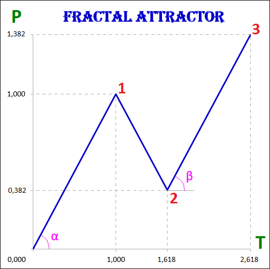
By fractal we mean the simplest attractor of oscillatory motion, consisting of three segments, of which one (2nd segment) is directed in the opposite direction to the other two (1st and 3rd segments).

Fractals are divided into types and types depending on the size of the cost and time intervals of their segments.

According to the property of self-similarity, fractals of a lower order form fractals of a higher order; accordingly, fractals of a higher order consist of fractals of a lower order.

3.5. The order, views and types of fractals.

Thus, any fractal, in addition to the cost and time values of the intervals, has the following characteristics that describe it:

1. The order of a fractal, indicating which segment it is in relation to fractals of a higher order and which segments of fractals of a lower order it is formed by itself.

2. The type of fractal.

3. View of the fractal.

Fractal structure, in this case, is the interconnection of fractals of different orders, types, types among themselves.

3.8. Basic fractal dynamics. 

3.9. Description of the fractal structure. 

The real market dynamics of the value of any financial asset is described by operator N. 

A basic fractal is one of the many fractals that form the fractal structure of the graphs of the dynamics of value, which are attractors. 

To describe the fractal structure of an attractor means to describe the types and types of fractals of its components, their sequence and location in relation to each other. 

The fractal structure of the attractor is both so complex and so simple that it is impossible to say what is more on the chart of quotations of financial assets - chaos or order. 

First, we will give a definition of chaos and order in a fractal structure, then we will describe the designation of fractals in a fractal structure, after which we will give their classification by types and types. 

3.10. Determination of order and chaos. 

A fractal is considered completed if all three of its segments are formed - the 1st, 2nd and 3rd. The completion of the 3rd segment indicates the completion of the entire fractal, since this is preceded by the sequential completion of the 1st and 2nd segments. 

In other words, order is discrete and chaos is continuous. The end of the 3rd segment of one fractal is replaced by the beginning of the 1st segment of another fractal of the same order or higher. 

Taking into account the fact that fractals of a lower order form fractals of a higher order, we can say that chaos and order are inseparable. 

Order is present in chaos and chaos is present in order. Chaos and order permeate each other and exist in one another. 

The dynamics of value in the financial market can be characterized as both chaotic and orderly. But chaos itself is nothing more than an order of the highest level, because nothing chaotic happens, since the graph of this dynamics is an attractor of a dynamic fractal determined by the operator N. 

3.11. The order of fractals. 

Each fractal is the first, second, or third segment of another fractal, which has a higher order. 

For an accurate description of the location of fractals in a fractal structure, their designation is required, the assignment of certain numbers to the fractals, which makes it possible to unambiguously understand which segments are fractals and what is their order in relation to other fractals. 

A fractal whose number consists of one digit is the highest fractal of the 1st order. 

A fractal whose number consists of two digits is a fractal of the 2nd order, of three - of the 3rd order, of four - of the 4th, etc. 

Fractals of the 4th order make up the fractals of the 3rd order, which in turn make up the fractals of the 2nd order, and those already constitute the fractals of the highest 1st order. 

3.12. Numbering of fractals. 

The highest 1st order fractal is numbered 1, 2 or 3 according to whether it is the first, second or third segment. A 1st order fractal consists of segments, which are 2nd order fractals. 

Fractal number 1 consists of segments numbered 11 (1st segment), 12 (2nd segment) and 13 (3rd segment). 

Fractal numbered 2 consists of segments numbered 21 (1st segment), 22 (2nd segment) and 23 (3rd segment). 

Fractal number 3 consists of segments numbered 31 (1st segment), 32 (2nd segment) and 33 (3rd segment). 

Fractals have the same order if they are either segments of one fractal that composes it, or are segments of other fractals, which in turn are segments of another fractal. 

A fractal is one order of magnitude less than another fractal if it is a segment of it. 

A fractal is one order of magnitude more than another fractal if that other fractal is a segment of it. 

A fractal indicated by a number is similar to a point indicated by coordinates, which is easy to find in the corresponding coordinate system. In our case, the coordinate system is a fractal structure. 

So, for example, if the coordinates of the fractal are number 132, then this means that this fractal is the 2nd segment of the 2nd order fractal with the number 13, which in turn is the 3rd segment of the 1st order fractal with the number 1. 

3.13. Determination of extremum points. 

The dynamics of value in the financial market is an alternation of uptrends and downward trends with the formation of local and global extremum points on the charts. 

From the point of view of the fractal structure of charts, extreme points (points where trends change) are points at which some fractal segments complete their formation and others begin to form. 

3.14. Views and types of fractals. 

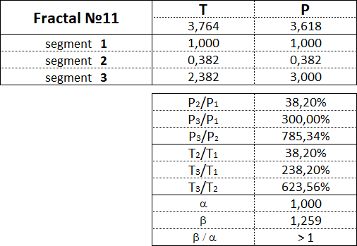
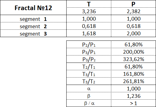
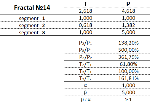
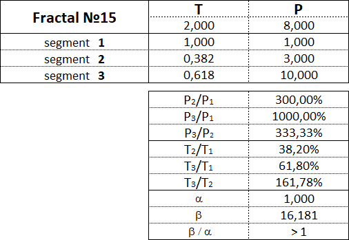
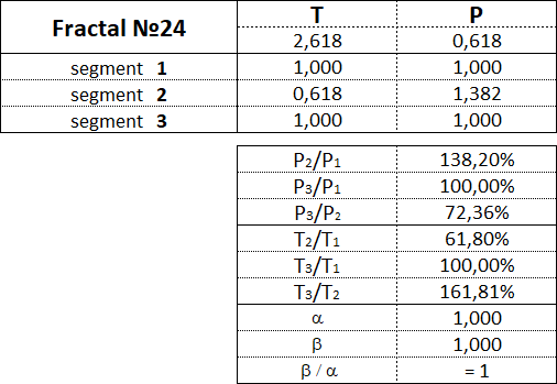
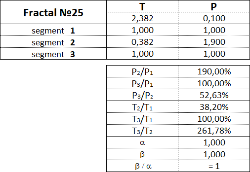
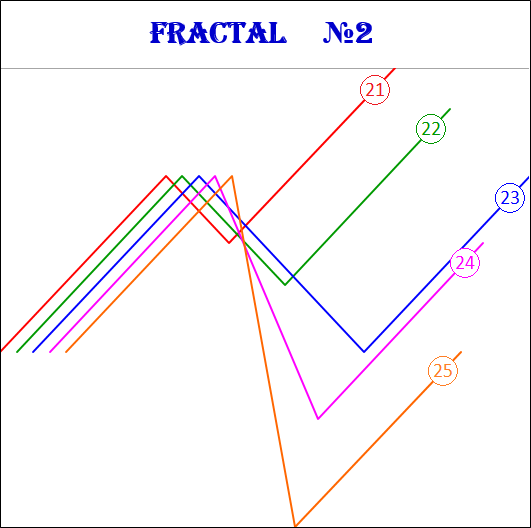
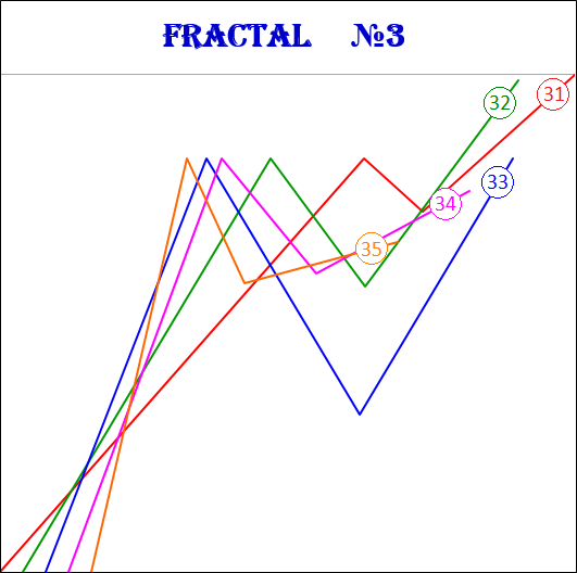
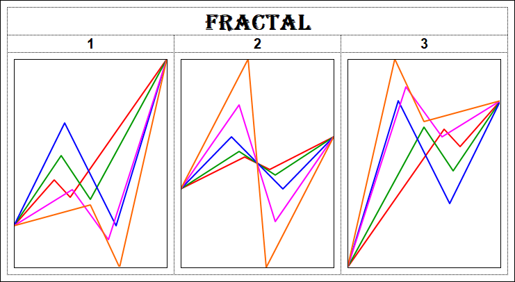
The fractal has three segments - the first, second and third. The second segment of the fractal is always directed in the opposite direction to the first and third segments. 

In addition to the order, which also indicates the segment number, each fractal segment has two characteristics (two parameters) - the price P (cost interval) and time T (time interval). 

P is a value characteristic that shows the length of the projection of the fractal segment onto the price axis, thereby denoting the price interval in which the segment was formed. 

T is a temporal characteristic showing the length of the projection of the fractal segment on the time axis, thereby indicating the time interval that it took to form the segment. 

A fractal consisting of three segments has six characteristics - these are P1, P2, P3, T1, T2, T3: 

• P1 and T1 - price and time intervals of the 1st segment; 

• P2 and T2 - price and time intervals of the 2nd segment; 

• P3 and T3 - price and time intervals of the 3rd segment. 

The main fractal is the basic fractal, the cost and time parameters of the segments of which are related to each other in the following proportions: 

1st proportion: 

P1/P3 = T1/T3 = 1; 

2nd proportion: 

P2/P1 = T2/T1 = 0.618. 

By changing the values of the parameters of the basic fractal using the Fibonacci coefficients using the golden section, we get a set of fractals that can be classified by views and types. 

Three views of fractals can be distinguished from the ratio of the cost parameters of the 1st and 3rd segments. 

View No. 1 - these are fractals in which the price interval of the third segment is greater than the price interval of the first segment: 

P1 < P3; 

View No. 2 - these are fractals in which the price interval of the third segment is equal to the price interval of the first segment: 

P1 = P3; 

View No. 3 - these are fractals in which the price range of the third segment is less than the price range of the first segment: 

P1 > P3. 

Regarding each view of fractals, we can say that the 2nd type of fractals characterizes the normal dynamics, the 1st type of fractals characterizes the dynamics with acceleration, and the 3rd type of fractals characterizes the dynamics with deceleration. 

From the ratios of cost and time parameters of the 1st, 2nd and 3rd segments, five types of fractals can be distinguished in each form. 

Three views and five types give 15 fractals, including the basic one. 

Fractals of the 1st view are designated by the following numbers: 

11, 12, 13, 14, 15. 

Fractals of the 2nd view are designated by the following numbers: 

21, 22, 23, 24, 25. 

Fractals of the 3rd view are designated by the following numbers: 

31, 32, 33, 34, 35. 

The first digit in the number indicates the view of fractal - 1st, 2nd or 3rd, and the second digit in the number indicates the type of fractal - 1st, 2nd, 3rd, 4th or 5th. 

Let's consider each of the 15 fractals separately and denote the proportions between the values of the cost and time intervals of its constituent segments. 

Let's start with the fractals of the 1st view, continue with the fractals of the 2nd view and finish with the fractals of the 3rd view. 

3.15. 15 fractals: 

3.15.1. Fractals of the 1st view. 

Fractals of the 1st view have the following numbers: 11, 12, 13, 14, 15. 

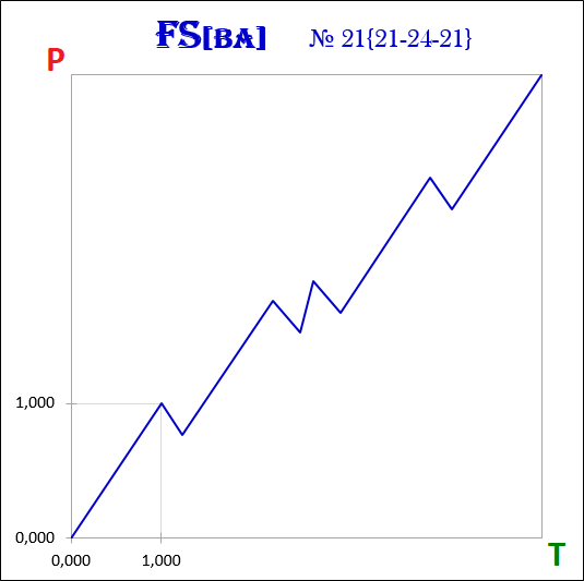
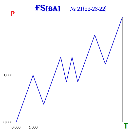
3.15.2. Fractals of the 2nd view. 

Fractals of the 2nd type have the following numbers: 21, 22, 23, 24, 25. 

3.15.3. Fractals of the 3rd view. 

Fractals of the 3rd type have the following numbers: 31, 32, 33, 34, 35. 

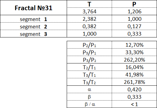
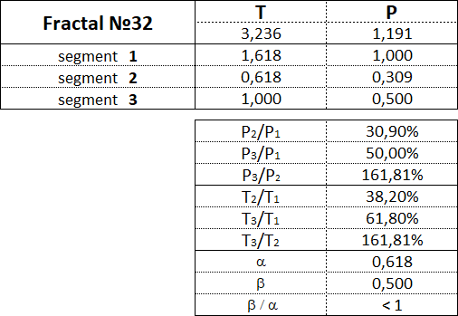
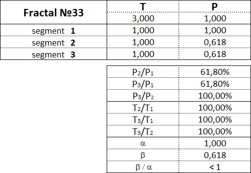
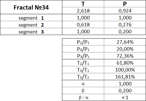
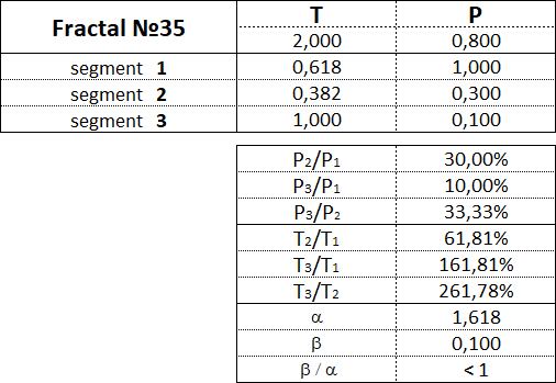
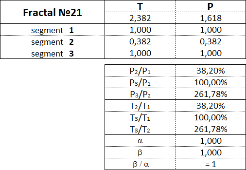
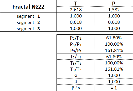
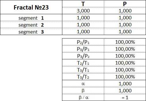
3.16. Proportions between fractal segments. 

This table shows the ranges of values as a percentage between the cost and time parameters of the segments for each of the 15 fractals. 

3.17. The Alphabet of Niro attractors.

From 15 fractals, you can make up a kind of alphabet of 15 letters.

As in the Morse code, with combinations of two symbols - dots and dashes, you can write any text, and in the alphabet of Niro attractors with combinations of 15 fractals, you can describe any fractal structure FS of any basic asset BA.

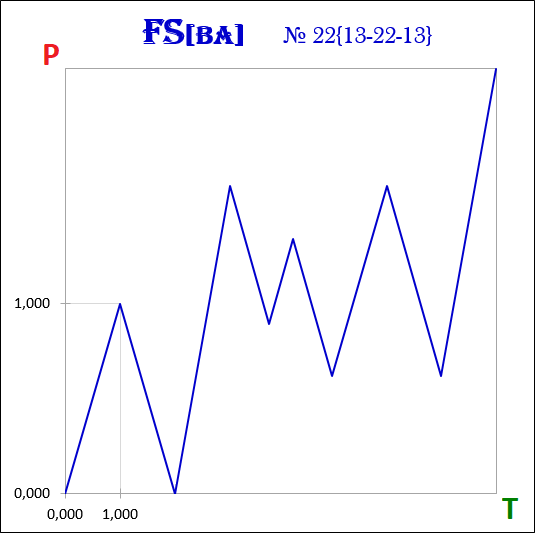
3.18. Bifurcation point and degrees of freedom.

A nonlinear dynamic system remains in chaos until a fractal is formed in the fractal structure of the chart. A formed fractal means that the system has passed from a chaotic state to an ordered state. The order that emerged from chaos will be disturbed by the beginning of the formation of a new fractal in the opposite direction to the already formed one, and the system will return to a chaotic state.

At the moment of completion of the fractal, a nonlinear dynamic system is at a bifurcation point, at which the system has several degrees of freedom - several options for the further development of its fractal structure. At the bifurcation point, it is possible to speak unambiguously only about a trend change, that is, a change in the direction of the future fractal to the opposite of the completed fractal, everything else - the cost and time intervals of future fractals, remains unclear, cannot be unambiguously defined.

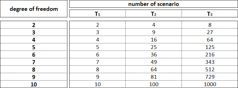
Let us consider an example of the formation of a fractal structure of a nonlinear dynamic system with two degrees of freedom at bifurcation points for three time intervals. A time interval is a period of time that is necessary for the formation of fractals of the same order.

The first development scenario is a scenario in which the cost interval of a new fractal does not exceed the cost interval of the completed fractal.

The second development scenario is a scenario in which the cost interval of the new fractal exceeds the cost interval of the completed fractal.

Let us denote by T0 the time interval for which the initial fractal was formed.

Then, in the T1 interval, two fractals can be formed, in the T2 interval - four fractals, and in the T3 interval - eight fractals.

The number of degrees of freedom at bifurcation points of a nonlinear dynamic system determines the number of possible scenarios for the development of its fractal structure in the current time interval, which with each subsequent time interval will increase exponentially.

The number of degrees of freedom at the bifurcation point of a nonlinear dynamic system is not constant and depends on its location in the fractal structure. 

A nonlinear dynamic system has the minimum number of degrees of freedom when the bifurcation point in the fractal structure is at the beginning of the formation of the smallest order fractal, which completes the largest order fractal. 

The maximum number of degrees of freedom falls on the bifurcation point that separates the completion of the highest order fractal and the beginning of the lowest order fractal. 

Taking this into account, modeling the fractal structure of a nonlinear dynamic system beyond the second time interval has no practical meaning due to the presence of a large number of possible scenarios for the development of a fractal structure. 

3.19. Cost and time intervals.

The fractal structure of the attractor is formed by dynamic fractals of various orders. At any moment in time, all fractals that form a fractal structure are at different stages of their completion - fractals of some orders can be fully completed, other orders - be in the initial stage of their formation, third orders - in the final, and the fourth - in an intermediate one.

Completed, i.e. formed, a fractal is a fractal in which all three of its segments are sequentially completed. Completion of the 3rd fractal segment is the completion of the entire fractal.

Completion of a fractal means the completion of the cost and time intervals of its segments.

The cost interval of a fractal is the interval between the beginning of the projection onto the price axis of the 1st fractal segment and the end of the projection of its 3rd segment.

The time interval of a fractal is the interval between the beginning of the projection on the time axis of the 1st fractal segment and the end of the projection of its 3rd segment. The time interval of a fractal is the sum of the time intervals of all three of its segments.

The strings of the fractal structure of the attractor are horizontal levels drawn through the extremum points formed in each month. The number of strings in a fractal structure is equal to twice the number of months it took to form it.

In the overwhelming majority of cases, the beginning and end of the cost intervals will be in the vicinity of the points lying on the strings.

The length of the cost interval is an absolute value, and the length of the time interval is a relative value.

Time is a form of the process of formation of a fractal structure and a condition for the possibility of its change.

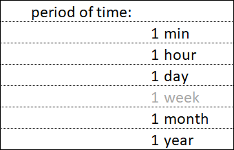
All these simple periods, except for the week, are multiples of each other. Thus, an annual period contains an integer number of monthly periods, a monthly period contains an integer number of day periods, a day period contains an integer number of hourly periods, and an hour period contains an integer number of minute periods. 

The time intervals of the formed fractals are located unevenly relative to simple time periods, but with a certain pattern. 

The beginning and end of a time interval can coincide with the beginning and end of a simple time period, but in the vast majority of cases, the beginning and end of time intervals fall in the vicinity of points that divide simple time periods along the golden ratio with Fibonacci coefficients of 0.382 and 0.618. 

In order to decompose the fractal structure of a chart into separate fractals with three segments, it is not enough to analyze charts that are built according to simple time periods - 1 minute, 1 hour, 1 day, 1 month, 1 year. To find the fractal structure, you need to analyze the charts that are built on all possible time frames. 

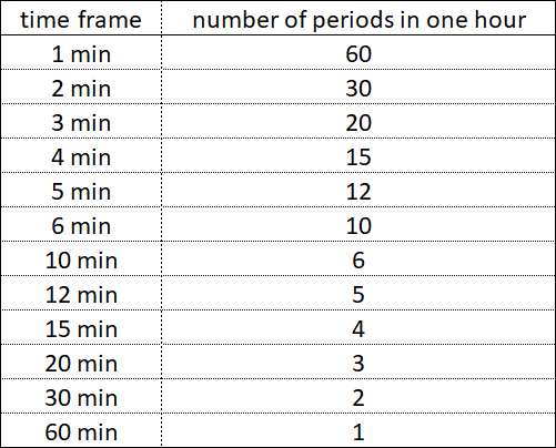
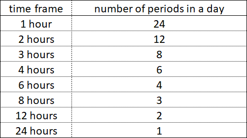
Within each simple period of time - whether it be 1 hour, 1 day or 1 year, there are smaller time periods, their components, which end simultaneously with each other at certain time intervals.

Within 1 hour, periods with time frames of 30 minutes, 20 minutes, 12 minutes do not end at the same time, but periods with time frames of 30 minutes, 15 minutes, 5 minutes in some time intervals end simultaneously.

Within 1 day, periods with time frames of 8 hours and 6 hours do not end at the same time, but periods with time frames of 8 hours, 4 hours, 2 hours or 12 hours, 6 hours and 3 hours in some time intervals end simultaneously.

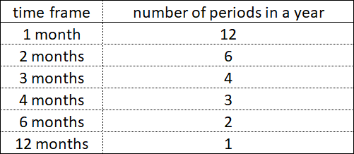
Within 1 year, periods with time frames of 4 months and 3 months do not end at the same time, but periods with time frames of 6 months and 2 months on some time intervals end simultaneously.

The periods of all time frames, starting at the same time, also end simultaneously at the end of the simple time period.

Low-order fractals form fractal structures on time intervals with daily time-frames, and fractal structures with fractals of even lower orders are formed on time intervals with hourly time-frames.

Higher order fractals form fractal structures on time intervals with monthly time frames, and higher order fractals form fractal structures on time intervals with annual time frames.

Completions of cost and time intervals occur at bifurcation points, which are in the overwhelming majority of cases on the strings of fractal structures. Taking into account the presence of a large number of degrees of freedom at bifurcation points in a nonlinear dynamic system, modeling the future fractal structure further than the second cost and time intervals leads to a huge number of models, often having the same probability of implementation, which does not allow choosing one single model as the most probable for implementation.

A more accurate prediction of the future dynamics of the value of financial instruments is achieved by analyzing and modeling the fractal structure of their charts between two bifurcation points closest to each other, i.e. only in the current cost and time intervals - in the direction of the formation of either the 1st segment, or the 2nd segment, or the 3rd segment of the fractal.

For short-term forecasting of the dynamics of the value of financial instruments, it is necessary to simulate the fractal structure of charts, which are built on the minute and hour time frames.

For medium-term forecasting of the dynamics of the value of financial instruments, it is necessary to simulate the fractal structure of charts, which are built on daily and weekly time frames.

For long-term forecasting of the dynamics of the value of financial instruments, it is necessary to simulate the fractal structure of charts, which are built on monthly and annual time frames.

The forecasting horizon in all three variants will be the same - the current cost and current time intervals of the emerging fractal, i.e. forming its first, second or third segments.

But on charts with hourly time frames, the forecast horizon will be a period of several days or weeks, on charts with daily and weekly time frames, the forecast horizon will be a period of several months, but on charts with monthly and annual time frames, the forecast horizon will be there will be a period of several years and even decades.

The cost intervals of fractals, regardless of their order, tend to end at points that are either at points lying on the strings of the fractal structure, or at points located at a distance from the strings in accordance with the Fibonacci coefficients.

Time intervals of fractals, the order of which is lower than the highest, tend to completion in the vicinity of the end points of time intervals, which are located within simple time periods in accordance with the Fibonacci ratios.

The overlapping of the end points of the cost and time intervals of fractals form bifurcation points that predetermine the values of the future cost and time intervals of new fractals.

Forecasting the dynamics of value for a long-term period requires an analysis of fractal structures formed by fractals of the highest and highest orders, the formation of bifurcation points in which is different from the fractal structures formed by fractals of the order below the highest.

The completion of the time intervals of fractals of the highest and highest orders occurs in the vicinity of the points at which the maximum number of annual time frames ends simultaneously:

1, 2, 3, 4, 5, 6, 7, 8, 9, 10, 11, 12, 13, 14, 15, 16, 17, 18, 19, 20, 21, 22, 23, 24, 25, 26, 27, 28, 29, 30, 31, 32, 33 and 34.

Special attention should be paid to the simultaneous termination of annual time frames, among which there are Fibonacci time frames: 1, 2, 3, 5, 8, 13, 21, 34.

On a time interval from 1 year to 40 years, the maximum number of simultaneous endings of time frames is 8. 

There are 8 simultaneous endings in the 24th, 30th and 36th years. 

In 24 year the following annual time frames end at the same time: 

1, 2, 3, 4, 6, 8, 12, 24. 

In 30 year the following annual time frames end at the same time: 

1, 2, 3, 5, 6, 10, 15, 30. 

In 36 year the following annual time frames end at the same time: 

1, 2, 3, 4, 6, 9, 12, 18. 

Over the time period 1 to 2200, the number of simultaneous time frame completions in years 1 to 34 ranges from 1 to 18. 

18 is the maximum number of concurrent completions in this time frame, which occurs in 1680. This year, the following time frames are completed simultaneously: 1, 2, 3, 4, 5, 6, 7, 8, 10, 12, 14, 15, 16, 20, 21, 24, 28, 30. 

The number of simultaneous completions of time frames in the interval (1; 2200) from 1 to 9 is 93.09%, the remaining 6.91% is accounted for by the number of simultaneous completions from 10 to 18. 

The end of the time intervals of the highest order fractals occurs at the time intervals where the number of simultaneous time frame completions ranges from 10 to 18. 

A summary of the simultaneous completion of time frames in years 1 through 34 for the period 1 through 2200 is shown in the graph and table below.

When analyzing the time intervals of fractals of the highest orders, the unfinished year is rounded up to the completed one, which does not allow making the analysis more accurate. 

To analyze time intervals with an accuracy of a month, it is necessary to construct, by analogy with the annual time frames, monthly time frames from 1 to 34 for the period from 1 year to 2100 and find the time intervals in which the maximum number of periods with different monthly ends at the same time frames. 

In this case, December 2000 would be a 24000 month, December 2100 would be a 25200 month, and July 2021 would be a 24247 month. 

The time interval 1-2100 contains 25'200 months. On this time interval, the number of simultaneous time frame completions in months 1 to 34 varies from 1 to 21 (21/34 = 0.618 - the “golden ratio”). 

21 is the maximum number of concurrent completions in this time interval, which occurs in the following years: 840, 1260, 1540, 1680, and 2100. 

The number of simultaneous completions of time frames in the interval (1; 25200) from 1 to 9 is 92.96%, the remaining 7.04% is accounted for by the number of simultaneous completions from 10 to 21. 

The end of the time intervals of the highest order fractals occurs at the time intervals where the number of simultaneous time frame completions ranges from 10 to 21. 

A summary of the simultaneous completion of time frames in months 1 through 34 for the period 1 through 2100 is shown in the graph and table below.

Let's designate the time interval as (1; L). where L ∈ N. 

ТF - time frame, time period repeating more than 1 time in the interval (1; L). TF ∈ N. 

m - simultaneous end of different time frames in the interval (1; L). m ∈ N. 

nm - the number of simultaneous endings of different time frames in the interval (1; L). n ∈ N. 

Earlier, the distribution of nm for TF = 34 was shown on two intervals for L1 = 2’200 and L2 = 25’200. 

The rise and fall of business activity shape the ups and downs in the economy, denoting economic cycles consisting of repeated recessions, depressions and revivals in the economy. 

The dynamics of the financial market takes place in correlation with economic cycles. Changes in the direction of dynamics of the values of stock indices, currency quotes, the cost of raw materials show the end of some economic cycles and the beginning of others. 

At the points at which time frames in years 1 to 34 end at the same time in the amount of more than 10 completions, there are changes in economic cycles. In the vicinity of these points, bifurcation points are formed in the fractal structure of the graphs of the dynamics of the value of financial assets in which some fractals end and others begin. 

To simulate the dynamics of economic processes, it is required to analyze the fractal structures of the charts, which are built according to the following annual Fibonacci time frames: 

1, 2, 3, 5, 8, 13, 21, 34, 55 and 10 years. 

The overlay of time intervals with the simultaneous completion of a large number of time frames from 1 year to 34th on time intervals with the simultaneous completion of a large number of timeframes from 1 month to 34th gives a clear understanding of where the time intervals of fractals will end of the highest order. 

Simultaneous endings of time frames within a time interval occur on specific dates, which are counted from the beginning of the interval. 

The modern chronology originates from the year in which he was born on Earth in a human body in one of his three hypostases - the Son of God, our God Jesus Christ. 

There are no clear and unequivocal facts confirming the birth of our God Jesus Christ in the very year from which the modern chronology is based. However, for Faith and for the salvation of the human soul, it is not the year of Birth that is important, but the Immaculate Conception and Birth of Jesus Christ, His Life and His Teachings, His Crucifixion and His Suffering, His Resurrection from the dead and His Ascension. 

There are many arguments pointing to the birth of the Son of God Jesus Christ 5 years earlier than it is commonly believed. 

Taking into account the uncertainty regarding the beginning of the modern chronology, for the analysis of the simultaneous completion of the annual intervals in order to identify the time intervals on which the global bifurcation points are formed, this fact must be taken into account. 

Given this fact, the current year 2021 could be the year 2026. 

Let's build the annual time frames from 1 to 144 (12²) and find the time intervals on which there is the maximum number of their simultaneous completions, paying special attention to those time intervals where the Fibonacci time frames end and paying attention to the difference between the time intervals equal to 5 years.

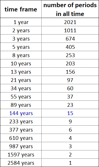
The vertices of the indicated parabolas are located in the vicinity of the time interval from 2021 to 2026. Taking into account the generally accepted time calculation, the upper limit of the range corresponds to the current year 2021. If the time is from 5 BC, then the current year is 2026, which corresponds to the lower end of the range. 

Given the lack of complete clarity about the beginning of the modern chronology, a situation is obtained in which the current time is either at the beginning of the 2021-2026 range, or at its end. 

The time interval 2021-2026, in which the vertices of the indicated parabolas fall, is an interval in the vicinity of which the maximum possible number of time frames ends in years from the 1st to the 144th, which indicates the completion of higher-order fractals in this time interval. 

The time range 2021-2026, in the vicinity of which + - 2 years, ends 56 time-frames, is followed by the year 2040, in which 23 time-frames end at the same time, which indicates the end of the time intervals of fractals of the highest orders.

2021-2026 is the time of the beginning of the end. Higher-order fractals that began in this period will complete the highest-order fractals by 2040.

2040 is a milestone year, after which new fractals of higher and higher orders will begin to form in fractal structures.

3.20. The essence of the modeling method.

At this, with time intervals, you can finish and complete the theoretical part by designating the essence of the method for modeling the dynamics of the value of financial assets, which consists in identifying the fractal structure of the financial asset graph and describing it using attractors from the Niro alphabet.

The process of formation of the fractal structure of the attractor by dynamic fractals is cyclical, which means it is predictable, i.e. it is possible to simulate the future dynamics of quotations of any financial instruments.

In the graphs of the dynamics of value in the financial market, there is a cycle, which consists in the formation of a fractal and is expressed in:

1. Formation of the 1st segment of the fractal.

2. Formation of the 2nd fractal segment directed in the opposite direction to the 1st.

3. Formation of the 3rd segment of the fractal, which has the same direction as the 1st.

After completing this cycle, the exact same cycle begins, but in the opposite direction. All these actions continue indefinitely - the first segment is always replaced by the second segment, the second segment is always replaced by the third segment, and the third segment is always replaced by the first segment.

The cyclical nature of the process of formation of fractals and fractal structure in accordance with a certain order gives an understanding of which segment of the fractal and in which direction will be formed after the formation of the current segment is completed.

At any moment in time, the dynamics of the value of any financial asset is in the formation of one of the three fractal segments - the first, second or third. After the first segment of the fractal, the second segment of the same fractal is always formed, after which the third segment of the same fractal is always formed and then the first segment begins to form again, but already of another fractal, which has either the same order or a larger one, and which is necessarily directed in the opposite direction the previous fractal.

The extreme points on the chart are the points at which either the first segments end and the second begin, or the second segments end and the third begin, or the third segments end and the first begin. The extremum points define the boundaries of the cost and time intervals of fractals in the fractal structures of attractors.

The proportions between the values of the cost and time intervals of the segments allow you to determine:

• what segments are they - the first, the second or the third,
• what kinds and types of fractals these segments form, and
• what is the order of the formed fractals in the fractal structure in relation to each other.

The method of modeling the dynamics of quotations of financial instruments is based on determining what the current fractal segment is - the first, second or third, in order to determine which segment of the fractal will be the next after the current one.

The alphabet of Niro attractors consists of 15 fractals:

11, 12, 13, 14, 15; 21, 22, 23, 24, 25; 31, 32, 33, 34, 35;

which are divided into three types, each of which has five types.

Each of the 15 fractals is an attractor to which the graph of any nonlinear dynamical system will strive.

Modeling the future dynamics of value begins with the analysis of the main fractal structure, consisting of fractals of the highest order, that is, with the analysis of charts built on annual time frames. As part of the analysis of the main fractal structure, it is determined to which of the 15 types of attractors the graph of the dynamics of the value of a financial asset belongs.

Having identified the attractor of the main fractal structure, it is possible to make not only long-term forecasts of the value dynamics, but also medium-term and short-term forecasts, because the formation of fractal structures consisting of fractals with an order below the highest will occur in strict accordance and subordination to the main fractal structure.

Thus, in order to clearly see the future dynamics of the financial market, it is necessary to know the alphabet of Niro attractors and be able to use it to read and describe fractal structures of charts of financial instruments traded in the currency, stock and commodity markets.

The Niro alphabet excludes apophenia from the dynamics of the financial market and makes the pattern in the dynamics of the value of financial assets clear and obvious. In this case, everyone can become a clairvoyant.

At this point, consideration of the main aspects of the method for modeling the dynamics of value in the financial market can be completed, from the theoretical part to move on to the practical and consider the application of the method of modeling future dynamics on a specific example.

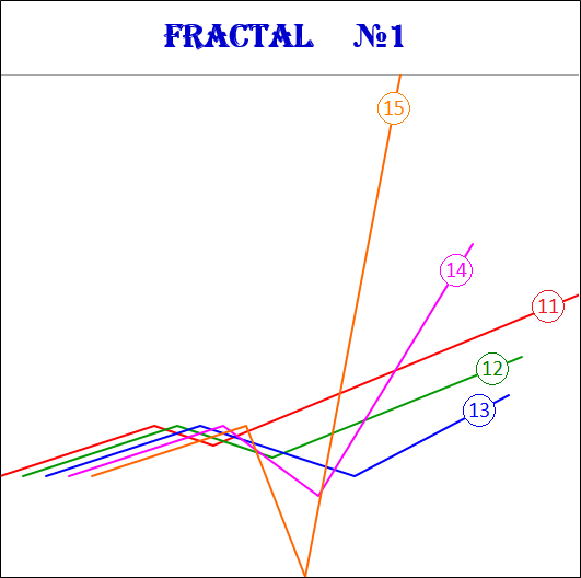
4. Model of the future dynamics of the Dow Jones index values.

As an example of modeling future dynamics, let us take the dynamics of the values of the American stock index Dow Jones.

Detailed and detailed modeling of the dynamics of the Dow Jones index is discussed in the article "When will Dow be Low?", and here is an already built model of the future dynamics, which has the highest probability of implementation at the moment.

1. Fractal F1333 is a fractal of the 4th order, it consists of segments: F13331, F13332, F13333, which are fractals of the 5th order and can be Fractal No. 23 from the Niro alphabet: 

F1333 ≡ F23. 

Forecasted time interval T1333 - (2014, 2035). 

Forecasted cost interval P1333 = 19750.86. 

2. Fractal F133 is a fractal of the 3rd order, it consists of segments: F1331, F1332, F1333, which are fractals of the 4th order and can be Fractal No. 11 from the Niro alphabet: 

F133 ≡ F11 → FS {13, MS, 23}. 

Forecasted time interval T133 - (2001, 2035). 

Forecasted cost interval P133 = 27164.66. 

3. Fractal F13 is a fractal of the 2nd order, consists of segments: F131, F132, F133, which are fractals of the 3rd order and can be Fractal No. 11 from the Niro alphabet: 

F13 ≡ F11 → FS {11, MS, 11}. 

Forecasted time interval T13 - (1978, 2035). 

Forecasted cost interval P13 = 34354.76. 

4. Fractal F1 is a fractal of the highest 1st order, consists of segments: F11, F12, F13, which are fractals of the 2nd order and can be Fractal # 11 from the Niro alphabet: 

F1 ≡ F11 → FS {13, 23, 11}. 

Forecasted time interval T1 - (1896, 2035). 

Forecasted cost interval P1 = 35,062.90. 

The 5th order fractal F13331 began to form in October 2014 and finished forming in May 2021. F13331 is the 1st segment of the 4th order fractal F1333, after the completion of which the fractal F13332 will begin to form, which is the 2nd segment of the F1333 fractal, and then the F13333 fractal, which is the 3rd segment of the F1333 fractal. 

The second segment F13332 of the fractal F1333, having begun to form in May 2021, may complete its formation in 2028. As part of the formation of the F13332 fractal, the Dow Jones index values may fall by 2028 to the level of 16,000 points. 

The 3rd segment F13333 of the fractal F1333 can form in the time interval from 2028 to 2035. As part of the formation of the fractal F13333, the Dow Jones index values may rise again from the 16,000 point mark to the 36,000 point mark. 

Fractals F13333, F1333, F133, F13 are the third fractal segments in which the order of each subsequent fractal is one order higher than the previous one. 

With the completion of the 5th order fractal F13333, the simultaneous completion of the 4th order fractal F1333 and the 3rd order fractal F133 and the 2nd order fractal F13 and the highest 1st order fractal F1 will occur. 

The 2nd order fractal F11 is the 1st segment of the highest 1st order fractal F1. F11 formed in the time interval from 1896 to 1973. 

The 2nd order fractal F12 is the 2nd segment of the highest 1st order fractal F1. F12 formed over the time frame from 1973 to 1978. 

The 2nd order fractal F13 is the 3rd segment of the highest 1st order fractal F1. F13 will form in the time interval 1976 to 2035. 

Thus, the attractor of the fractal structure FS {13, 23, 11} of the Dow Jones index graph is the F11 fractal - fractal No. 11 from the Niro alphabet, which is of the 1st type and belongs to the 1st type. 

Completion of the F13 fractal in 2035 will complete the F1 fractal. Thus, the cycle of growth in the Dow Jones index, which began in 1896, will end. 

In 2035, a global downtrend will begin in the American stock market. The fall in quotations of American stocks may be so strong that the value of the Dow Jones index will drop to the level of 2700 points. This decline will take place within the formation of the highest order fractal F2, which is the second segment in the global fractal structure. 

5. Conclusion.

In conclusion, I would like to note that a person, in a sense, is a complex biological nonlinear dynamic system that produces other nonlinear dynamic systems, including such as the financial market.

The future behavior of nonlinear dynamical systems is always multivariate, that is, at any moment of time there are always several alternative attractors of these systems. There is never one single scenario for the development of certain events, either in a person's life or in the financial market.

Those events that occur in a person's life now, and those actions that a person commits now, respectively determine the events that will occur in the future, and the actions that will be performed in this future by him.

Those fluctuations in value in the financial market that are occurring now and those fractals that are formed on the charts of financial assets now directly determine their future dynamics.

The human brain is a biological computer that functions in strict accordance with the programs and algorithms loaded into it, which form its worldview, which determines its life, views, actions, actions.

The method of modeling the value in the financial market, which was discussed above, can be considered a kind of computer program, well, or a kind of algorithm, having “loaded” your brain with which, you can see and understand that nothing random and chaotic happens in the financial market and that the dynamics of quotations financial assets is ordered and defined by the operator N.